This software and documentation was developed within the context of the
EUMETSAT satellite Application
Facility (NWP SAF). The partners in the
NWP SAF are the Met Office, ECMWF, KNMI, and Météo-France.
Appendix B. Minimization

Here the observations, y, have error covariances R; B is the error covariance matrix of the a priori (background) profile x0; and y(x) is the observed radiance that would result for a given atmospheric state x.
Rodgers (1976) gives three variations of iterative solution to the minimisation of J(x), two of which are:

and

where xn
is the nth estimate of the atmospheric profile
(the background profile being the 0th estimate) and
 .
.
Equation (2a) is the more efficient version when there are more profile elements than channels (i.e., R is smaller than B). However, when there are more channels than profile elements the form in Equation (2b) should be used.
In Rodgers's paper, Eqn. 2a above is Eqn 101, while Eqn. 2b is Eqn. 100. Therefore in this code, when the minimisation is to be done using the former method NWPSAF_Minimise_101 is called while NWPSAF_Minimise_100 is called in the latter case.
Equation (2b) also differs from (2a) in that it can also be extended to allow for extra terms in the cost function (e.g., to penalise solutions with supersaturated levels or with superadiabatic lapse rates) and can be modified to become the Marquardt-Levenberg descent algorithm (Rodgers, 2000). This case is dealt with in the NWPSAF_Minimise_100ML subroutine
The Marquardt-Levenberg version of Eqn. (2b) with the additional cost function terms is then:

Here J' is the first differential of the additional cost function with respect to x, evaluated at xn, and J'' is the second differential. Thus, J' is a vector with the same length as xn and J'' is a matrix with the same size as B.
In the Marquardt-Levenberg minimisation method, the value of ![]() is varied
depending on the non-linearity of the problem and the proximity to the
desired solution. When
is varied
depending on the non-linearity of the problem and the proximity to the
desired solution. When ![]() , the equation reduces to the
Newtonian inverse Hessian method of Eqn (2b). In non-linear cases, it
is possible that the step taken by using the Newtonian method will
result in an increased cost function. In this case the value of
, the equation reduces to the
Newtonian inverse Hessian method of Eqn (2b). In non-linear cases, it
is possible that the step taken by using the Newtonian method will
result in an increased cost function. In this case the value of
![]() is increased (thereby reducing the step size) until a point is reached
where the cost function decreases (as
is increased (thereby reducing the step size) until a point is reached
where the cost function decreases (as ![]() , Eqn. (3) becomes the
method of steepest descent). After an improved solution (i.e., lower
cost function) has been found, the value of
, Eqn. (3) becomes the
method of steepest descent). After an improved solution (i.e., lower
cost function) has been found, the value of ![]() may once again be
increased to allow larger steps in the next iteration.
may once again be
increased to allow larger steps in the next iteration.
The NWPSAF_Minimise subroutine allows for either the Newtonian or Marquardt-Levenberg algorithms to be used and for the inclusion of additional cost function terms.
In all cases the minimisation is implemented by solving Eqn. 2a, 2b
or 3 without explicitly inverting the matrix. This achieved through the
use of the Cholesky Decomposition method of solving linear symmetric positive
definite systems of equations (e.g.,
Golub and van Loan, 1996, p.143ff).
Convergence is deemed to have occurred when:
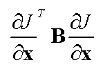
The cost function gradient is normalised using the B-matrix as a metric:
In the case where the cloud top pressure and cloud fraction are being retrieved
(with very large assumed bacground error variances), the appropriate elements
of the cost function gradient are set to zero. The cost function gradient is
not calculated and is set to zero if Eqn. 2a is being used for minimisation.
The manipulation of the observational error covariance matrix in its
various forms (see Section 2.2.4) requires some additional code in all
four of the routines considered in this section. For the band diagonal
case (except for diagonal matrices which are trivial to manipulate), further
subroutines are called to invert and multiply the matrix. The inversion
of a band diagonal matrix is handled by the
NWPSAF_Band_Inverse subroutine
which uses a Band Cholesky routine in the process ( Golub and van Loan,
1996, pp.155-6).
[ Return to Top ]
Golub, G.H. and C.F. Van Loan (1996). Matrix Computations.
The Johns Hopkins University Press.
Rodgers, C. D. (1976). Retrieval of atmospheric temperature and composition
from remote measurements of thermal radiation. R. Geophys. Space Phys.,
14, 609-624.
Rodgers, C. D. (2000). Inverse Methods for Atmospheres: Theory and
Practice. World Scientific Publishing.
![]() decreased in the previous iteration.
decreased in the previous iteration.

References.